The research group I work with has access to a small GPU cluster, which occasionally sits idle. To avoid wasting valuable compute resources (IDLE GPUs essentially burn money through opportunity costs), I decided to train a German GPT-2-style model from scratch, using only German text.
Existing German models available on Hugging Face have 137M parameters and a context length of 1024 tokens1, which is quite limited compared to recently released models, such as those in the LLAMA family.
After the training and writing the first draft of this article, I became aware of some larger German models, such as the
- LLäMmlein,
- Sauerkraut (by VAGO) and
- Bueble-LM series.
While the existence of these larger and more capable models probably means that the one presented here will not be used as much, I still enjoyed the learning experience.
To make the model at least somewhat competitive with current alternatives, I aimed to support context lengths of at least double that. I also wanted the model to have more parameters, which generally enhances model quality. Therefore, I set out to train a GPT-2-style model with 358M parameters and a context window of 2048 tokens. While still modest compared to state-of-the-art models, it’s an improvement. The resulting model is available on at kkirchheim/german-gpt2-medium.
Dataset §
A large dataset is required before training a model. Since this LLM is German-only, it was crucial to ensure that the collected texts were in German.
Selection §
While we could have scraped the internet ourselves to gather enough data, this would be a lengthy process, requiring a custom crawler seeded with relevant pages and a substantial runtime.
Thankfully, others have already done this work: Common Crawl provides a massive text dataset from internet scrapes spanning the past decade. A derivative project, the German Colossal, Cleaned Common Crawl corpus (GC4), contains the German subset of the entire Common Crawl. This means that we do not have to download the entire internet and filter for German content manually.
Since the data was scraped from 2015 to 2020, this will be the knowledge cutoff for our LLM. For context, existing German-only models were trained on just 90GB of text.2
While this dataset is publicly available, which is nice for reproducibility, the fact that it is a collection of scraped data also means that we do not have the licenses. For research purposes, it is allowed to train models on such content.3
Preparation §
To start, we downloaded all the .tar archives listed on the website - around 180GB of compressed text. After extraction, we are left with 300GB of uncompressed, high-quality German text in something similar to JSON format.4
We can inspect the resulting files with
head de_head_extracted/de_head_0000_2015-48.txt
which gives us something like
{
  "url": ...,
  "date_download": ...,
  "length": ...,
  "nlines": ...,
  "source_domain": ...,
  "title": ...,
  "language": "de",
  "language_score": 0.99,
  "raw_content": "Siegmar Gerber Titel:\nAnwendungslösungen zur Simulation von Rechenanlagen auf dem ZRA 1 und zur Bibliographieautomatisierung mit Hilfe des Rechners ODRA Erscheinungsdatum:\nIm Beitrag werden Lösungen für zwei Anwendungsprojekte beschrieben, die in den sechziger Jahren am Institut für Maschinelle Rechentechnik der Leipziger Universität mit Hilfe der Rechenanlagen ZRA 1 bzw. ODRA realisiert wurden."
}
Here, raw_content is the field that we are interested in, as it contains the extracted text from the scraped websites.
We can use the other fields to get some insights into our dataset, and filter for higher-quality content.
So, first, we filter all entries where the language score < 0.98, which makes sure that our dataset only contains german webpages.
Then, we can investigate the source of the articles, by counting the values of the source_domain column:
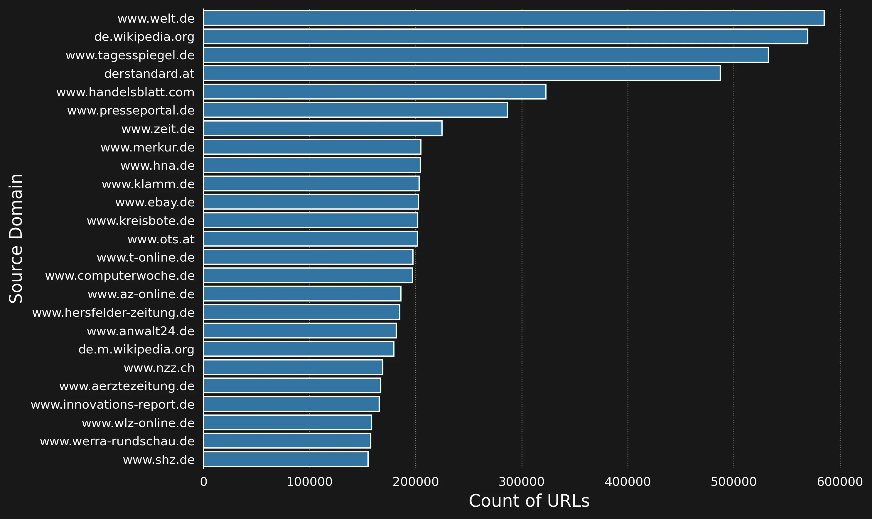
Article Sources
As we can see, the dataset contains mostly news sites and Wikipedia. Furthermore, we can inspect the length of the articles:
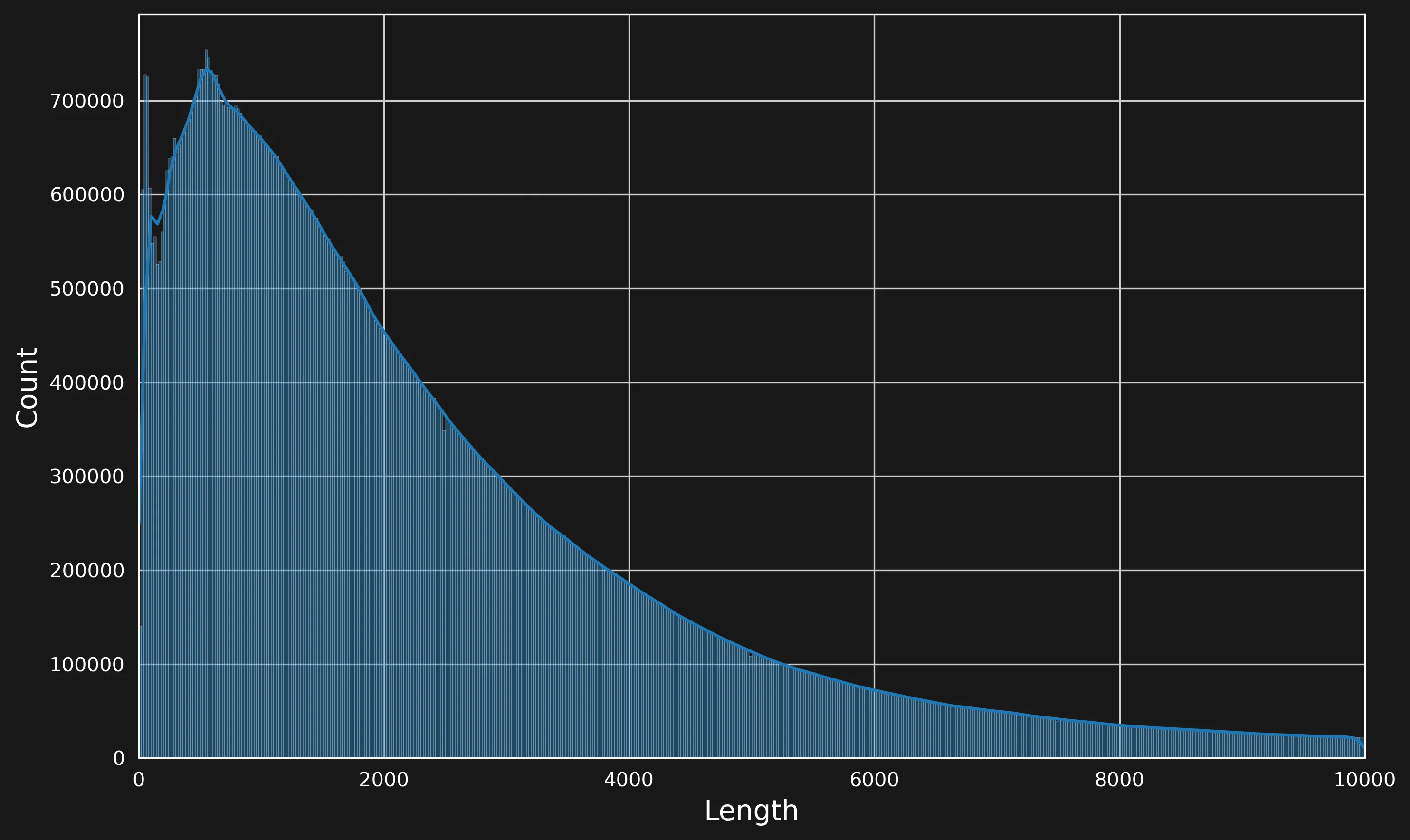
Distribution of length of articles (in characters)
We store the filtered dataset as JSON, discarding all fields apart from raw_content.
This allows us to directly load the datasets using the Huggingface datasets library:
from datasets import load_dataset

dataset = load_dataset(
    'json',
    cache_dir="./cache",
    data_files=['de_head_extracted/*.json'],
    split="train"
)

print(f"Length: {len(dataset)}")
This tells us that there are 117,412,577 texts in total. After loading everything, the cache will be 1.2T in size.
Training §
Training an LLM involves two main steps: first, creating a tokenizer to map character sequences to tokens that the LLM can process (and vice versa). Second, training the LLM to predict a probability distribution over the next tokens, given preceding tokens in the text.
Tokenization §
Training a tokenizer with Hugging Face is quite straightforward5, and I gave it a try. However, in the end, I opted to reuse the tokenizer used of stefan-it/german-gpt2-larger:
from transformers import AutoTokenizer

tokenizer = AutoTokenizer.from_pretrained("stefan-it/german-gpt2-larger")
tokenizer.pad_token = tokenizer.eos_token
There are better tokenizers available that, as far as I know, differ mainly in how they deal with numerals.
We tokenize the entire dataset, caching the results on disk:
# Tokenize the dataset and count tokens in one step
def tokenize_and_count(examples):
    tokenized = tokenizer(
        examples["raw_content"],
        truncation=True,
        max_length=2048
    )
    tokenized["num_tokens"] = [len(t) for t in tokenized["input_ids"]]
    return tokenized

# Tokenize and count in a single step
tokenized_dataset = dataset.map(
    tokenize_and_count,
    batched=True,
    num_proc=128,
    cache_file_name="cache-tokenized/.tokenized_dataset_cache"
)

total_tokens = sum(tokenized_dataset["num_tokens"])
print(f"Total number of tokens: {total_tokens}")
This tells us that the entire dataset has 66,537,920,947 tokens.
The num_procs=128 parameter significantly speeds up the process, from 24h to < 1h.
We can then split the dataset into a training and a validation portion.
# Split the dataset into train and validation sets
train_val_split = tokenized_dataset.train_test_split(test_size=0.0001)

# Get the train and validation sets
train_dataset = train_val_split['train']
val_dataset = train_val_split['test']
Model Configuration §
As described earlier, we want to train a gpt-medium-model, but with increased context size. How do we do this?
In Huggingface, models are described by config.json configuration files that parameterize the architecture.
The original configuration for a gpt2-medium looks like this:
{
  "activation_function": "gelu_new",
  "architectures": [
    "GPT2LMHeadModel"
  ],
  "attn_pdrop": 0.1,
  "bos_token_id": 50256,
  "embd_pdrop": 0.1,
  "eos_token_id": 50256,
  "initializer_range": 0.02,
  "layer_norm_epsilon": 1e-05,
  "model_type": "gpt2",
  "n_ctx": 1024,
  "n_embd": 1024,
  "n_head": 16,
  "n_layer": 24,
  "n_positions": 1024,
  "n_special": 0,
  "predict_special_tokens": true,
  "resid_pdrop": 0.1,
  "summary_activation": null,
  "summary_first_dropout": 0.1,
  "summary_proj_to_labels": true,
  "summary_type": "cls_index",
  "summary_use_proj": true,
  "task_specific_params": {
    "text-generation": {
      "do_sample": true,
      "max_length": 50
    }
  },
  "vocab_size": 50257
}
The documentation for these hyperparameters is here. There are a couple of modifications that we have to make:
- n_positions: the maximum number of tokens that the model can be used with, which we adjust to 2048
- n_ctx: this is the actual context length, so we set it to 2048 as well.
We then put the modified config.json this into a directory called mymodel and create the model with:
cfg = GPT2Config.from_pretrained("mymodel")
model = GPT2LMHeadModel(cfg)
Optimization §
After everything is set up, we can use the Hugging Face API to train the model. The API makes this extremely convenient.
Given the corpus size and the limited resources, I only trained for a single epoch.
date_time = datetime.now().strftime("%m%d%Y-%H-%M-%S")

training_args = TrainingArguments(
    output_dir='./results',
    num_train_epochs=1,
    learning_rate=6e-4,
    per_device_train_batch_size=12,
    gradient_accumulation_steps=12,
    per_device_eval_batch_size=12,
    gradient_checkpointing=True,
    warmup_steps=1000,
    torch_compile=False,
    weight_decay=0.1,
    logging_dir=f'./logs/{date_time}',
    logging_strategy="steps",
    disable_tqdm=False,
    report_to="tensorboard",
    save_total_limit = 3,
    logging_steps=10,
    fp16=True,
    ddp_find_unused_parameters=False,
    dataloader_num_workers=32,
    optim="adamw_torch",
    resume_from_checkpoint=True,
    eval_strategy="steps",
    eval_steps=100
)

cb = TextGenerationCallback(tokenizer=tokenizer, log_dir=f"./logs/{date_time}")

trainer = Trainer(
    model=model,
    args=training_args,
    train_dataset=train_dataset,
    eval_dataset=val_dataset,
    data_collator=data_collator,
    callbacks=[cb]
)

trainer.train()
We run the training script with
torchrun --nproc_per_node 4 train.py
If the training crashes, you can resume by using
trainer.train(resume_from_checkpoint="results/checkpoint-xxx")
Monitoring §
Once the training runs, we can use different tools to monitor the process.
nvtop §
nvtop displays the utilization of the GPUs.
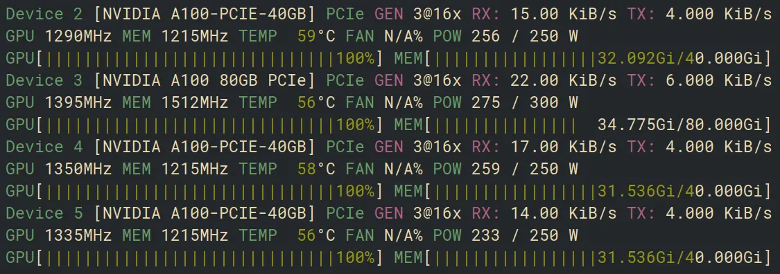
GPUs go BRRRRR
This way, we can, for example, determine whether the process allocates sufficient VRAM or if there is still space to increase the batch size.
Tensorboard §
The trainer prints statistics to the terminal at regular intervals. However, Tensorboard provides a web interface to watch training statistics in real time.
Tensorboard can be enabled by the report_to="tensorboard" argument in the training configuration.
The web interface can then be launched by executing:
tensorboard --logdir logs/
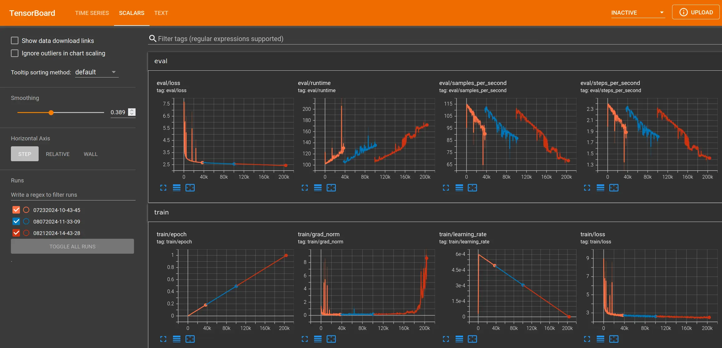
Live training statistics in Tensorboard
By implementing a custom TextGenerationCallback, we can sample from the GPT during training.
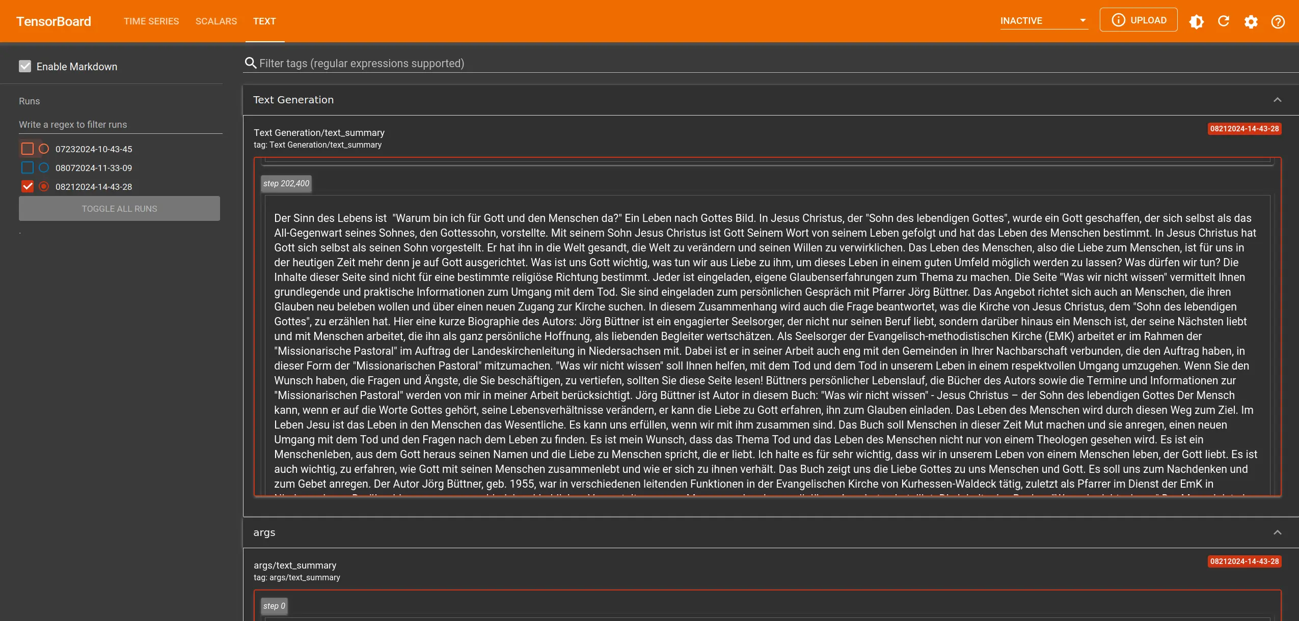
Live text samples in Tensorboard
Plotting §
We can also download statistics in JSON format from Tensorboard to process them programmatically.
The loss curve over the training period is shown below. Aside from some initial spikes, it follows the expected pattern: a sharp loss drop at first, followed by a gradual decrease as training progresses.
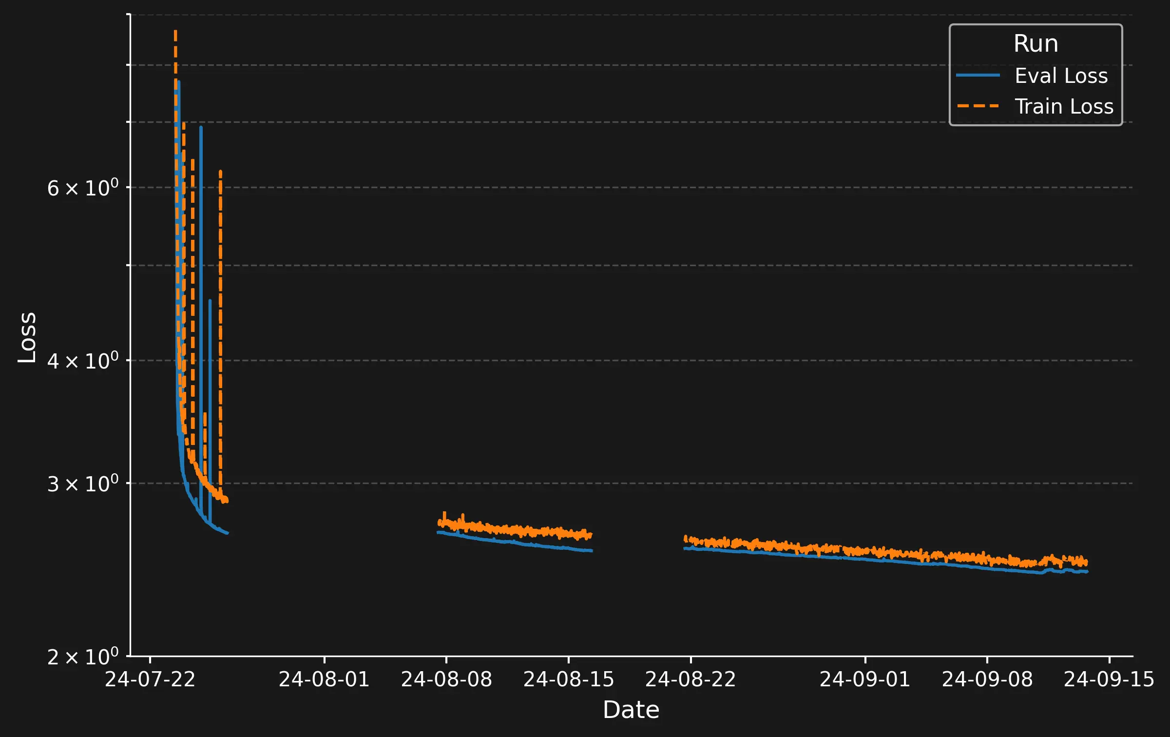
Loss over Training. The gaps in the data indicate crashes of the training script.
Gradient Norm Spikes §
During training, we can observe an interesting phenomenon: when we look at the norm of the gradient of the loss $\lVert \nabla_{\theta} \mathcal{L}(x, y) \rVert$ w.r.t. the models weights $\theta$, we see (plot below) that
- they start at around $1$ and then quickly decrease. However, we observe some spikes, particularly in early epochs. These spikes also correlate with some drastic jumps in the model’s loss (see image above).
- we can see that the gradient norm increases towards the end of the epoch.
This magnitude tells us something about how large the updates are that we apply to the model’s weights. It makes intuitive sense to me that we start out with quite large updates at the beginning of the training, and then gradually move towards the minimum of the loss in smaller steps as it becomes more difficult to improve the loss, so the gradient is not as steep.
However, to be honest, I do not know why we observe these jumps and the gradual increase towards the end of the epoch. If you have any suggestions, feel free to contact me.
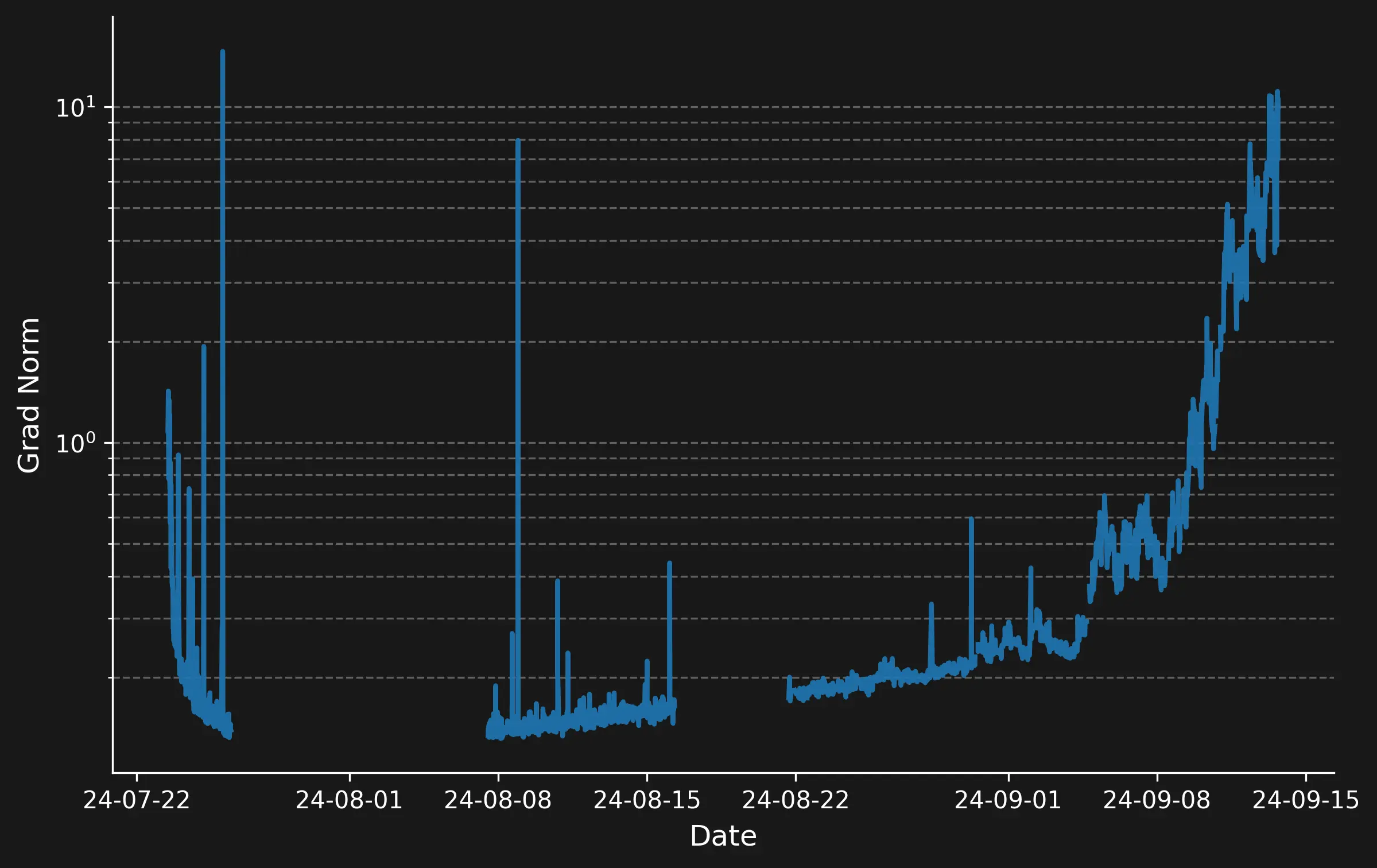
Spikes in the norm of the gradient
Evaluation §
Now that the model is trained, how can we evaluate it?
Qualitative §
One of the first things we can do to assess how good (or bad) the model is, is to simply have a look at some example generations. For example, we make the model complete the following text:
from transformers import pipeline

pipe = pipeline("text-generation", model="kkirchheim/german-gpt2-medium", device="cuda")

text = pipe("Der Sinn des Lebens ist",
            max_length=256,
            no_repeat_ngram_size=3,
            top_k=50,
            top_p=0.95,
            do_sample=True
 )[0]["generated_text"]
print(text)
The result looks like this:
Der Sinn des Lebens ist der Weg in die Freiheit, die wir für uns und unsere Kinder anstreben.
Das Wichtigste dabei ist es, die richtige Entscheidung für eine Lebens- und Sozialform zu treffen.
Denn nur wenn Kinder in einer Familie aufwachsen und Familie ihr Leben selbst bestimmen können, werden sie sich auch in Zukunft in ihrer Persönlichkeit verwirklichen. Wie wichtig es ist, in einer gesunden und lebenswerten Umwelt zu leben, zeigt sich am großen Anteil von älteren Menschen. Der demografische Wandel ist in vielen Bereichen bereits spürbar und wird viele Menschen immer stärker belasten.
Viele Familien in unserer Region leben seit Generationen im Eigentum. Sie sind in einem Generationenverbund mit ihren Kindern mit ihren eigenen Bedürfnissen und Ideen an den Ort ihrer Wohnumgebung gebunden. Die Generation der Jüngeren lebt zu einem Großteil allein in einer kleinen Wohnsiedlung ohne eigenen Garten, im Altersheim oder als alleinstehende Rentnerin oder Rentner.
Die Lebensbereiche Wohnen, Familie und Gesellschaft rücken in dieser Situation in den Fokus der Gesellschaft und erfordern die Entwicklung von neuen gesellschaftlichen, sozialen und ökonomischen Lebensmodellen.
Mit unserer Gesellschaft und unseren Kindern ist es oft nicht mehr so einfach wie früher, in dieser Lebensphase, sich von einer festen Bindung in die neuen Lebensphase zu lösen. Neue soziale Systeme müssen deshalb ganz neu entwickelt werden, um
While this reads strange, at times, it does resemble valid German text.
Language Modeling §
For English models, there is a plethora of benchmarks that evaluate all kinds of properties of the model, such as its reasoning abilities, its knowledge in certain fields, or its truthfulness. However, for German text, our choices are quite limited. However, what you can always do is to compare the losses of different models on the same corpus. This will give you an idea of how well the models can predict the next token. Instead of comparing the loss, people often compare the per-token-perplexity, which is a measure of how perplexed the model is by a given text. Perplexity over a sequence of tokens $w$ with length $N$ is computed as: $$ PPL(w) = \exp \left( -\frac{1}{N} \sum_{i=1}^{N} \log(p_{\theta}(w_i \mid w_1, …, w_{i-1})) \right) $$ so, in essence, it is the exponentiated loss.6 In practice, perplexity is often only approximated, as computing it exactly requires $N$ forward passes, which can take a very long time for larger corpora.
There are several implementations of the perplexity metric available online, and interestingly, many of them give slightly different results. So, I went with the implementation of higgingface evaluate, which I only modified slightly, because it would throw an error for some of the models.
For the evaluation, we took the first 10k articles of german Wikipedia.
from datasets import load_dataset

dataset = load_dataset("wikipedia", "20220301.de", split="train")
text = [sample['text'] for n, sample in enumerate(dataset) if n < 10000]
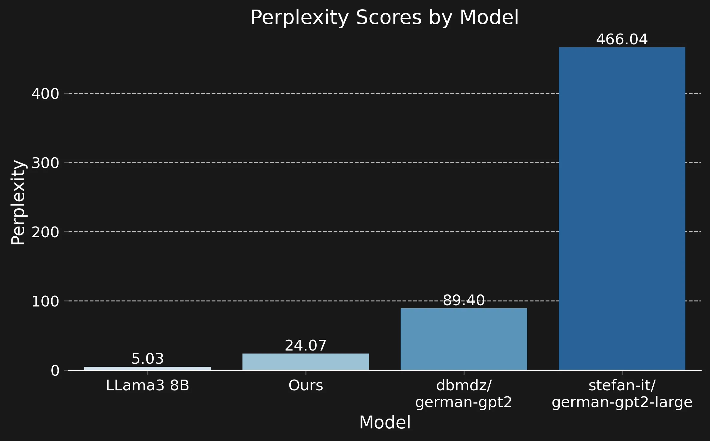
Perplexity of different models on some test data
As you can see, the LLama model outperforms ours, which is unsurprising, given that it has over $20 \times$ the number of parameters. Our model, on the other hand, outperforms the smaller German models (also, unsurprisingly, as it is larger and was trained on much more data). It should be noted that per-token perplexity can be difficult to compare between models with different tokenizers, so I am not entirely sure how to interpret the performance difference to LLama3. However, the German models all use the same tokenizer.
I am not entirely sure why the stefan-it model performs so poorly.
According to the model card, it is basically a variant of the dbmdz model trained on much more data, so you would expect it to perform better.
Memory Footprint §
Model quantization can be used to reduce the VRAM required for inference. The table below shows the maximum required GPU memory for generating 1024 tokens.
As we can see, our model requires more RAM compared to the model of stefan-it (and, similarly, dbmdz, which has the same architecture), but is still significantly less RAM intensive than the Llama model.
| Quantization Level | Ours | stefan-it/ german-gpt2-larger | meta-llama/ Meta-Llama-3-8B |
|---|---|---|---|
| fp32 | 2242.32 | 641.44 | 31218.98 |
| fp16 | 1174.63 | 341.87 | 15614.70 |
| int8 | 910.54 | 260.32 | 8970.10 |
| int4 | 771.42 | 219.27 | 6126.09 |
Inference Speed §
Full Precision §
Measuring the time that each model requires to generate 1k tokens on an A100 reveals that our model is approximately two times slower compared to the smaller stefan-it, but still twice as fast as the Llama model.
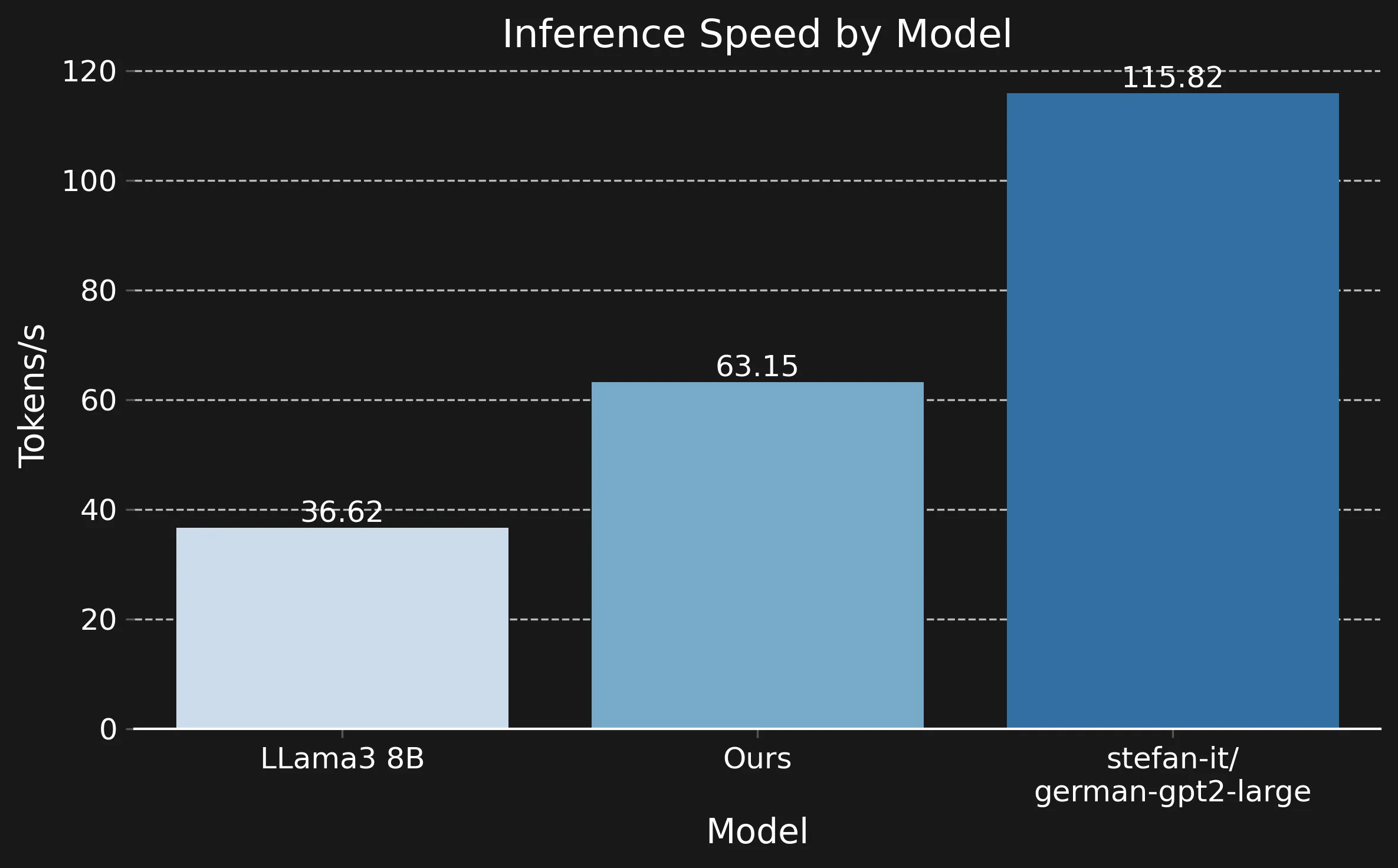
Generated tokens per second on an A100
Quantization §
While one could assume that quantization also accelerates inference (as I did), this does not seem to be the case. Below, you can see a histogram depicting the distribution of time required to sample 1024 tokens from our model on an A100. We use histograms since this allows us to additionally inspect the distribution of values.
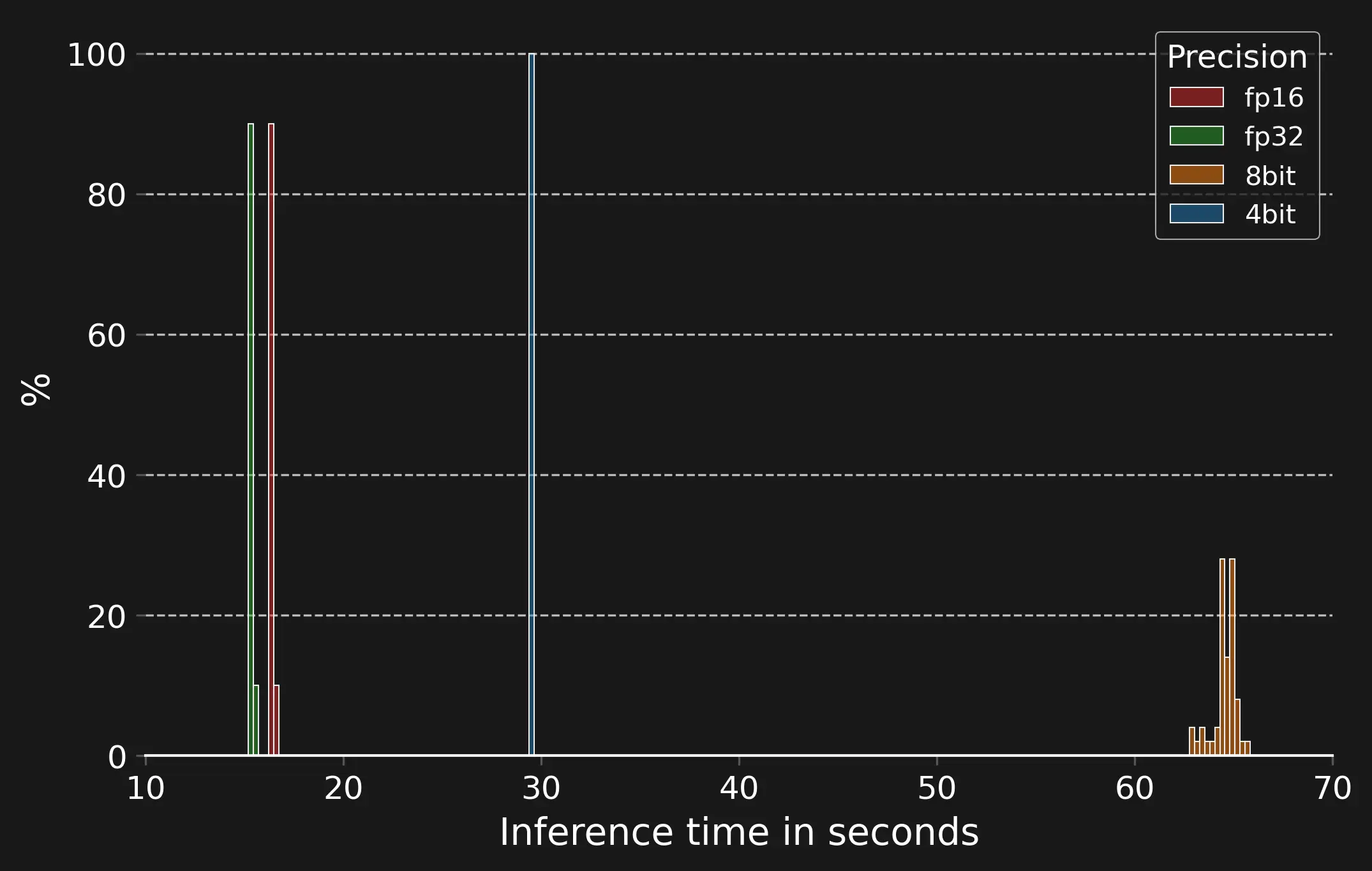
Time required to generate 1024 tokens with different levels of quantizations on an A100
Lessons Learned §
Throughout collecting data, implementing the training script and finally evaluating the model, there were several lessons which I learned.
Crashes Happen You might have noticed gaps in the previous plots. One key lesson I learned is that training can unexpectedly be interrupted, even when there’s no apparent reason. For instance, if the disk becomes full and the Hugging Face Trainer tries to save a new model checkpoint, it crashes. Without prior checkpointing, this can mean a lot of wasted compute.
Batch-Size Matters Initially, I started training the model with a moderate batch-size, however, it turns out that this leads to a loss plateau early on. In my search for solutions to this problem, I had a look the the hyperparameters in Kaparthys Nano GPT and noticed that this implementation uses much larger batch sizes.
To my knowledge, the largest and best purely German models are dbmdz/german-gpt2 and stefan-it/german-gpt2-larger. The latter is trained on the same corpus, but only on 90GB of the CommonCrawl. ↩︎
According to the information provided on huggingface. ↩︎
Concerning the EU AI act, which will be enacted soon, this is still legal for research purposes in Europe. I assume that the EU AI Act is the reason that some recently released LLAMA models are not available in the EU: Meta does not want to get sued. ↩︎
The format is not exactly JSON, but serialized Python. On the common-crawl website, there is example code that demonstrates how to load data in this format. ↩︎
There is an excellent post on perplexity available on the Gradient. There is also a paper describing alternative evaluation strategies. ↩︎
